Enhancing Data Visualization: Nested Ranks for Multiple Dimensions in Tableau

Mastering Nested Ranks: Advanced Techniques for Data Analysis in Tableau

Unleashing Insights: Leveraging Nested Ranks for Enhanced Data Representation in Tableau

Rank is a very powerful concept in Tableau and one of the widely used Table Calculations. It can be used in many situations along with other Helper functions like Index(), First(), Last() and Size(). It can also be very effectively leveraged for Pagination.

When building visualizations, the focus would be to show the best performing metrics/values. As seen in some of the other blogs, we have used different methods to prepare the Top N and Bottom N values. In this blog, we will focus strictly on the Top Ranks across multiple Dimensions within the same visualization for the same measure.  Though this can be easily achieved by placing multiple sheets on a Dashboard and providing a Drill down approach though action filters, it might not be an acceptable solution for all end users. This blog provides a step by step approach to solve this using Calculations and Table Calculations where all pieces are put together in a single visualization.

Understanding Nested Ranks in Tableau: A Comprehensive Guide

Implementing Nested Ranks for Multiple Dimensions in Tableau

Advanced Strategies: Enhancing Data Analysis with Nested Ranks in Tableau

Optimizing Data Visualization: Techniques for Effective Nested Ranks in Tableau

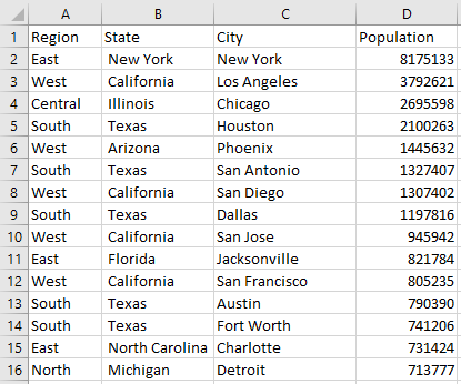
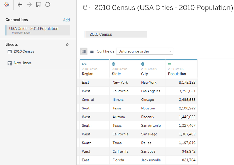
For this example, we will be using 2010 Population data for some of the cities across USA. We have taken 161 Cities, 25 States. For testing purposes, the data is split into 5 Regions: North, South, East, West and Central.

Harnessing Nested Ranks: Strategies for Improved Data Visualization in Tableau

Maximizing Insights: Advanced Techniques for Nested Ranks in Tableau

Elevating Data Analysis: Leveraging Nested Ranks for Actionable Insights

Empowering Decision-Making: Using Nested Ranks in Tableau for Deeper Insights

This blog will be approached more like a use case. The requirements are:

1. Show the Top Cities by Population and their Ranks.

This is very straight forward.

2. Show the Top Cities by Population within each State with their Ranks.

If the need was to show within a single state, it could have been easily achieved using a Context Filter. But we need multiple States to be displayed.

3. Show the Top States by Population within each Region with their Ranks.

Slightly getting complicated here because there is a need for Hierarchy Ranking.

4. Show Top Regions by Population and their Ranks.

This is the most complicated step as it requires double Hierarchy ranking or nested ranking within all the above-mentioned Dimensions.

5. Provide a single control for all three Ranks.

This step is achieved by a Parameter which can select all the three Ranks

The requirements look a little complicated at first, but as we slowly go into each of the pieces, it becomes better.

Though this example works in most cases, we need to be a little careful with the calculation when there is a Many : Many relationship (duplicate matches).

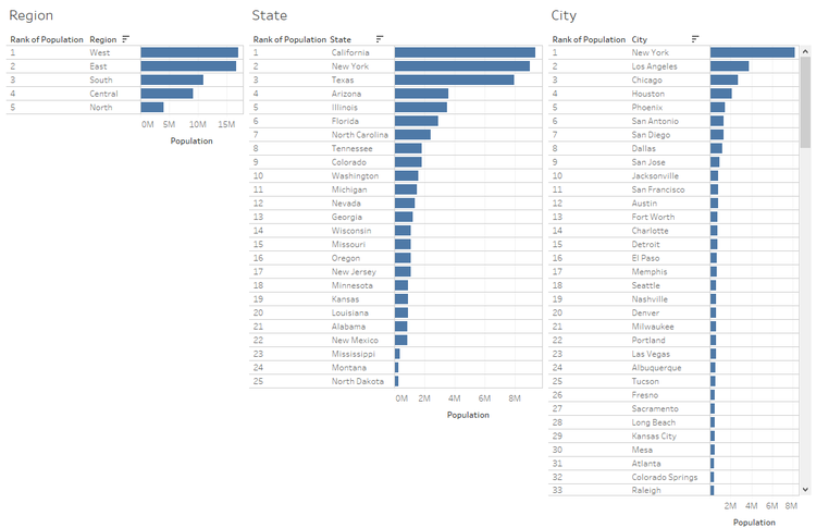
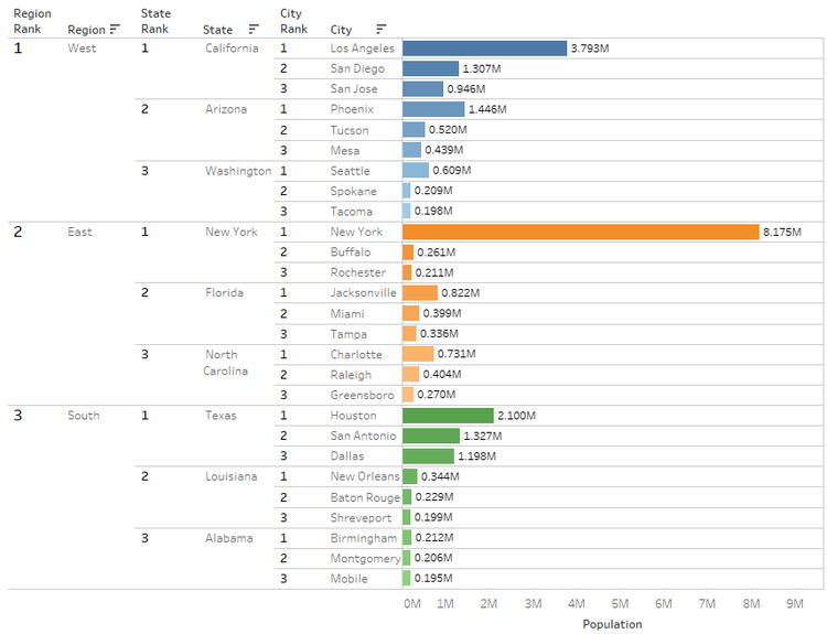
The concept is to combine all the three visualizations into one with Nested features as displayed in the image before.

We will go though the entire process step by step. We will start from the inner most Level of granularity i.e. City Ranks and slowly progress towards the outer pieces of the visualization which are more complicated.

Before we go into the steps, we need to understand the different types of Rank functions.

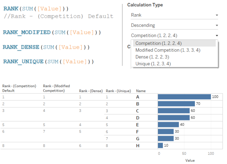
As we can see in the image, we have some repeated values. This is the focus area for the future steps.

a) Rank

This is the default calculation. It is the standard competition rank. When there are matching values, the next value will be incremented. In the first Column, Row 3 and Row 4 have the same rank. So, the Rank for Row 5 is incremented by 1.

b) Rank_Modified

As seen in the second Column, whenever there are matching values, that particular rank is skipped and incremented by 1. Row 3 and Row 4 have the same rank, so Rank 3 is skipped.

c) Rank_Dense

As seen in the third Column, matching values are given the same rank and all future ranks are also listed without skipping any value.

d) Rank_Unique

As seen in the fourth Column, every row gets a Rank irrespective of matching entries. The Rank is provided alphabetically. It works like the Index() function.

For our example, we will use Rank_Dense. This feature will be explained when we reach the step.

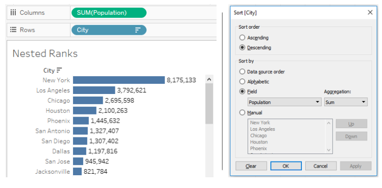
1) We will start with Population and City. This will be the innermost part. Any basic chart will work. Here we will go with a horizontal Bar chart with Labels. If needed, we can format the labels to M or K. Sort in descending order of Population

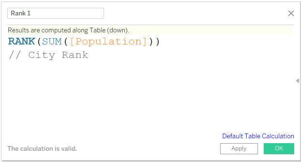
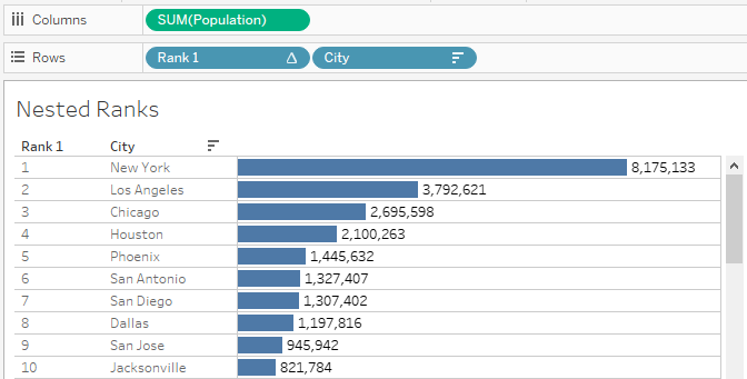
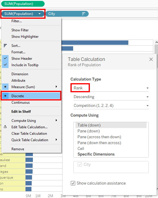
2) Creating the Rank. Here Rank and Rank_Dense, both will work as we do not have any duplicate values. We will use it as a Discrete field on Rows to the left of City field.

By default, all Table Calculations will be computed Table Across or Table Down. In this case, City is on Rows, so the Ranking will be Table Down. This will change in the next step. The field can be saved as an Adhoc calculation. It will be renamed as Rank 1 or City Rank.

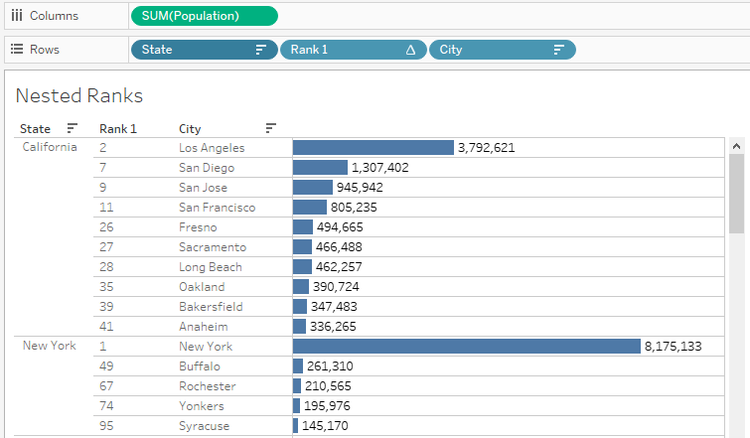
3) The next step would be to bring the State field as parent to the left. We do not need any Hierarchies here. Sort the States in Descending order of Population.

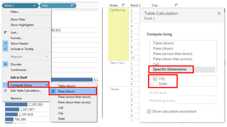
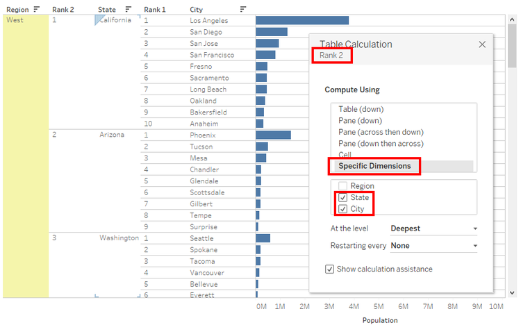
The Ranks are displayed for the entire dataset. We need to change it for each state. We can use the Pane Down option or Specific Dimensions, by deselecting the partition field.

** Every Table Calculation has two major features

a)       Type of Calculation – Running Calc, Window Calc, Percent, Rank etc.

b)      Scope and Addressing – Scope represents that partition or we can treat it as the pane. Addressing is the travel direction which can be treated as the granularity for which the value is calculated.

When we use the Specific Dimensions option, we need to read it as “For every Unchecked field (Partition – Scope) calculate the Table function for every Checked field (Direction – Addressing).

In this example, the function will be evaluated for every State.

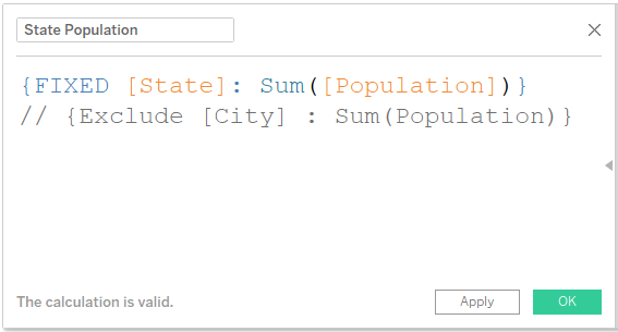
4) Next, we need to provide Ranks for State field. For this we need to know the values for each state. We can either use a Fixed LOD Calculation or an Exclude LOD Calculation. If we are using Fixed, we go with State. If we are using Exclude, we go with City.

We need to be a little careful when using Fixed calculation. If there are duplicates, it might cause an issue with overall aggregate values. For example Greenville as a city. It is present in multiple states in USA. Same goes with Springfield, Madison, Fairview etc. Our sample data is much cleaner. Also, we are not doing it at City level. So not an issue here.

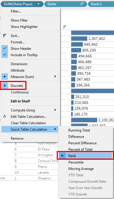
5) Next we need use this field as a Discrete field as shown in the second step and convert to Rank with default Scope and Addressing.

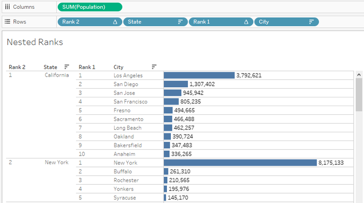
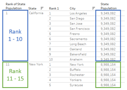
But here, we have an issue with the Rank. Since the Rank is Competition rank by default, the rank gets incremented. We need to repair it.

In the image, the state population is shown for better understanding. Since every row is a duplicate as per the Fixed Calc, the value will be repeated.

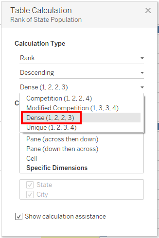
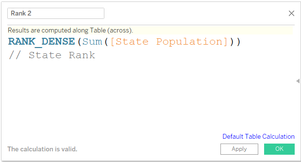
6) We need to convert the Rank into Rank_Dense.

The same can be done using a Calculated Field. The field can be called Rank 2 or State Rank.

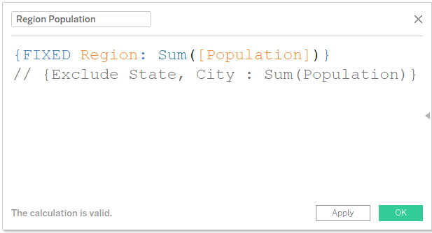
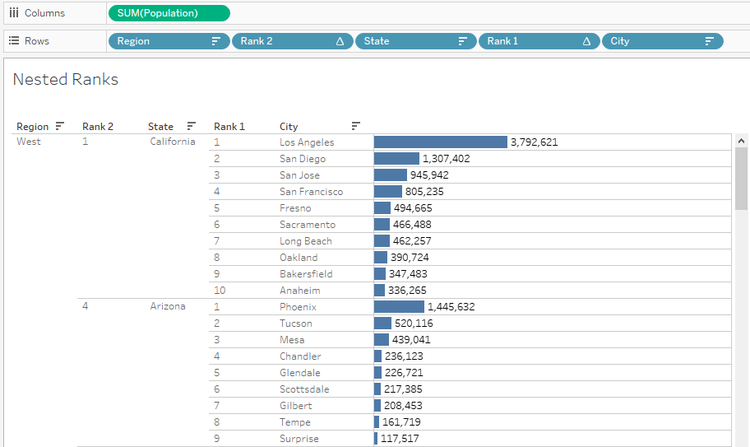
7) Next, we will introduce the Region field. All the steps that were used for State ranks have to be repeated for Region.

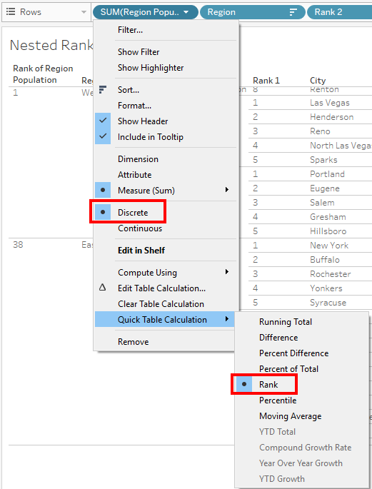
As soon as the Region is introduced, the State rankings change. We need to recompute the Ranking for each Region.

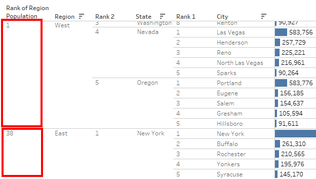
Now, for the remaining steps.

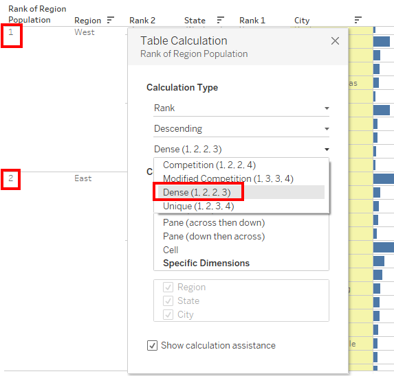
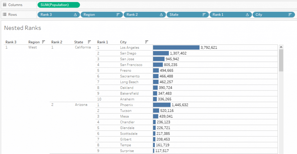
We can create a field and name it Rank 3 or Region Rank.

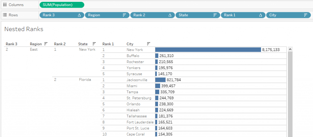
Now, we can see all Region wise Ranks and their nested values for two levels.

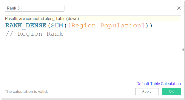
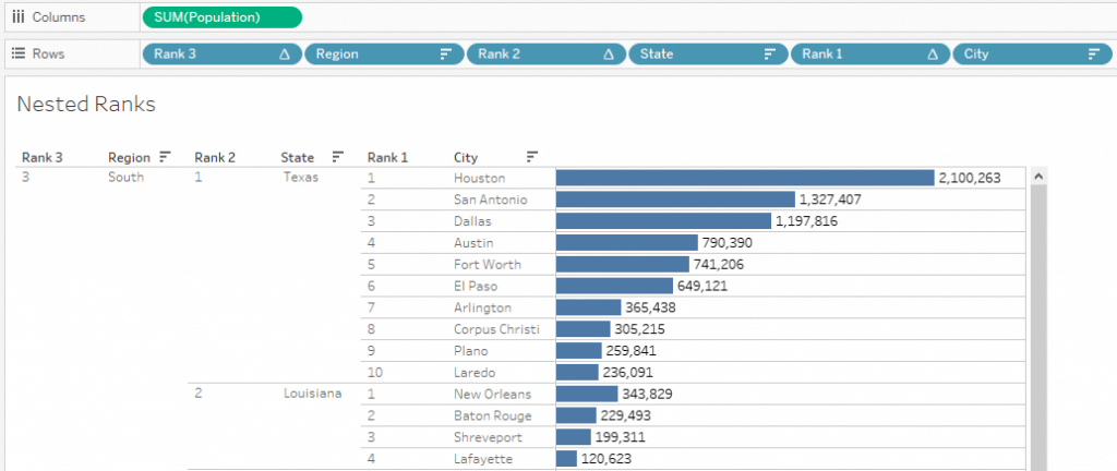
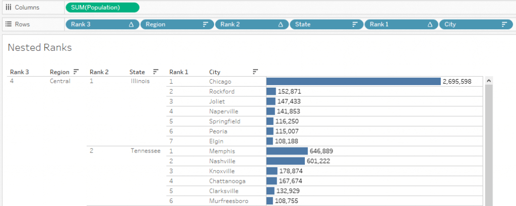
All the main requirements defined initially are accomplished at this point. Only the Parameter step is remaining.

Since there is considerable amount of data, scrolling up and down becomes a little tedious. We shall create a Top N parameter. Though we can create 3 different parameters and apply logic for all three, we will keep it simple and create one. For example, users might want to see the Top 3 Regions and Top 3 States within each Region and Top 3 Cities within each State.

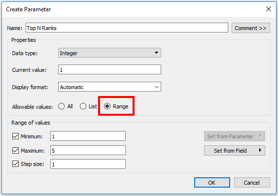
8) Creating the Top N parameter with a Range of Values 1 to 5 and showing the Control to the End User.

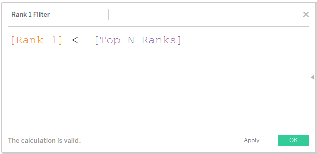
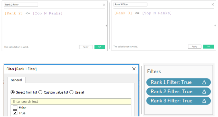
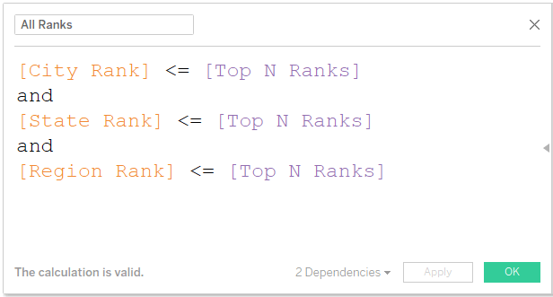
9) To activate the Parameter, we will create the logic. A simple Boolean function for all the Rank fields and using on the filter shelf with a True condition.

Or we can combine all logic statements into one single calculation. This field can be used on the filter and set to True.

Now we have all the features in place. We can start using the Parameter.

After adding some colors and changing formats, we arrive at this view