Unleash the Power of Infographic Designer in Power BI: Transform Your Data into Visual Stories

Crafting Compelling Visual Narratives: Exploring Power BI’s Infographic Designer Feature

Elevate Your Data Storytelling with Infographic Designer in Power BI

Introduction to Infographic Designer

Infographic designer chart provides the ability to display the data in form of multiples rows and columns. This chart makes use of a lot of shapes, icons and even play around with the colors. It represents the information in a way that best describes a story. It also has the flexibility to import personal icons and make use of them. For instance, using a single icon or stacked multiple icons to make a column or bar, it will give a column chart or bar chart in a pictographic way.

Introduction to Infographic Designer in Power BI

How to Use Infographic Designer: A Step-by-Step Guide

Customization Options and Best Practices for Infographic Designer

Examples of Infographics Created with Power BI’s Infographic Designer

Getting Started with Infographic Designer: Basics and Navigation

Designing Engaging Infographics: Tips and Tricks

Exploring Advanced Features of Power BI’s Infographic Designer

Harnessing the Power of Visual Storytelling: Infographic Designer in Action

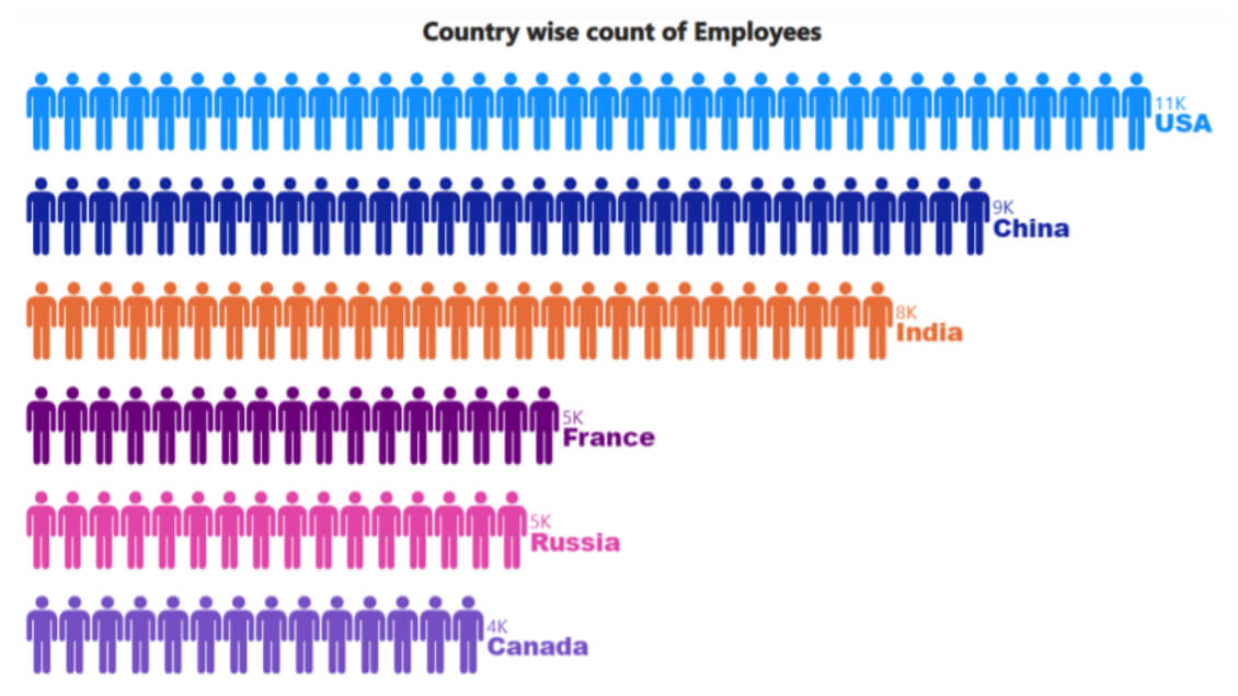
In this article, I have demonstrated how to build an infographic designer chart. Here, I have used a dummy dataset that has country wise number of employees for a particular company. Infographic designer will help your dashboard or reports to be visually beautiful, quickly understood, and easy to remember.

Step 1: Accessing the Infographic Designer Visual

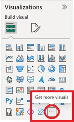
To get this visual, you can go to marketplace by clicking on the three dots i.e., ‘Get more visuals’.

Step 2: Importing and Placing the Visual on the Canvas

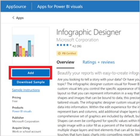
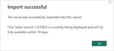
The marketplace will get opened. Search the visual i.e., ‘Infographic Designer’ and import it by clicking on ‘Add’ button.

As soon as the visual gets added, it will show the success message as below –  

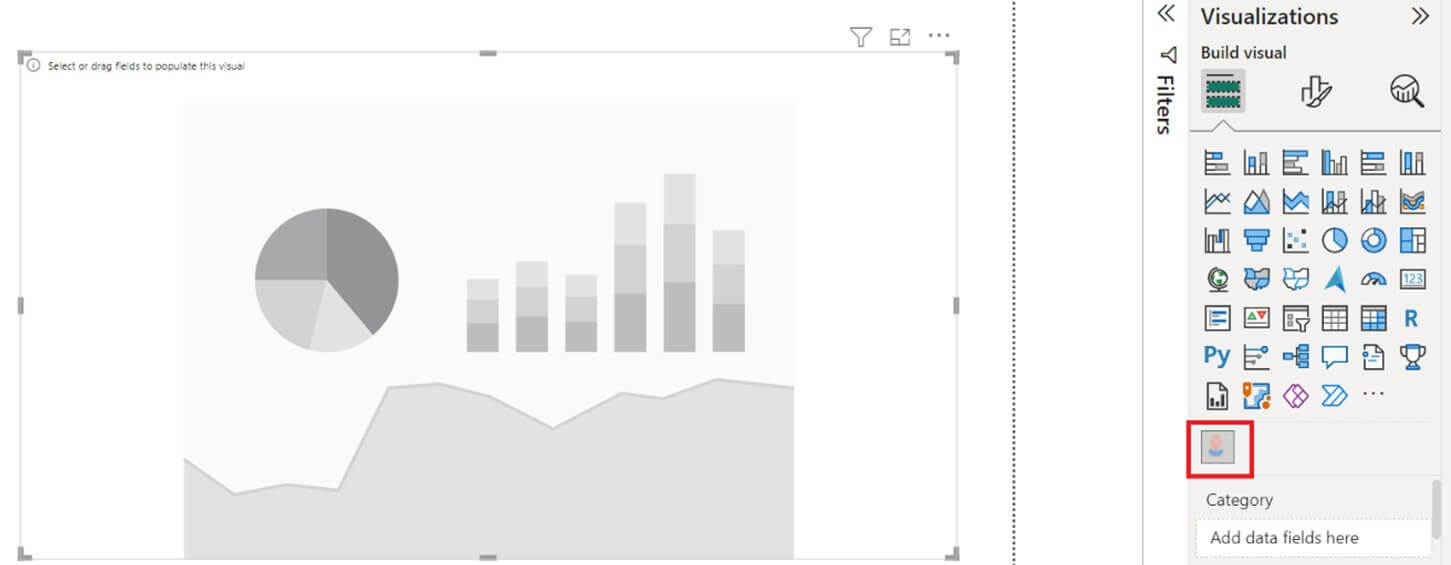
After this, you will be able to see the viz under the visualisation pane. Once it is there, you will have to place it on the canvas. 

Step 3: Setting up the Category and Measure Fields

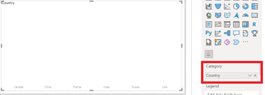
Now, drag the category column to ‘Category’ fields. Here, we have Country column as the category. You will see something like the below viz when you do that. 

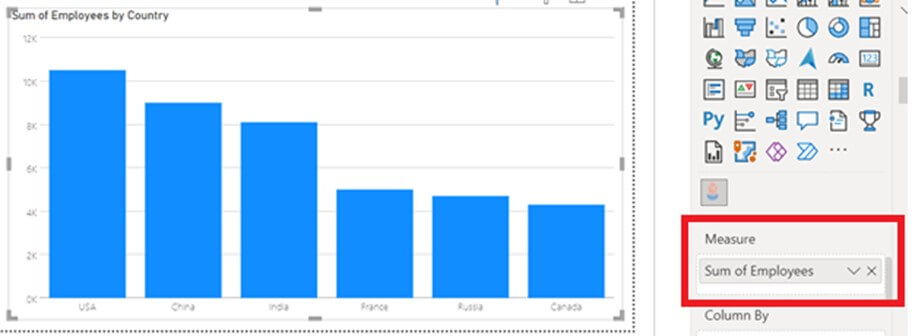
Drag the measure from the Fields pane and drop it to the ‘Measure’ field. Here, we have number of employees as the measure. You should see a bar chart by doing this. By default, it shows the vertical bar chart. 

Step 4: Formatting the Chart with Mark Designer

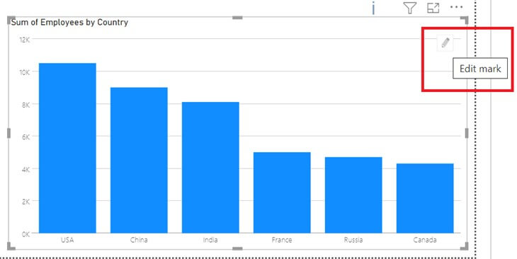
Now, all we will need to do is some formatting. For doing that, use the below highlighted icon.  

Step 4.1: Editing Shapes and Colors

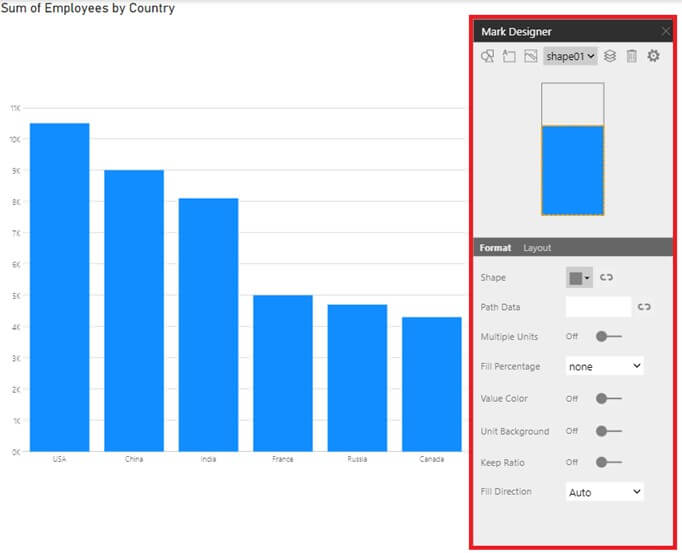
After clicking on the ‘Edit Mark’ icon, you will see a new pop-up box on the chart with the name ‘Mark Designer’. This will allow you to edit the chart according to the preferred requirement.  

This has some additional settings like adding the category on X-axis, Y-axis or even adding the data label, adding the color to it, and changing the format of the same. Also, you can add/remove/edit the shapes and color them accordingly. There can be more than 1 shape and more than 1 text. 

Now, we will start with doing some formatting to this chart. 

We already have ‘Shape01’ that has the bars for each category type. Any shape added will be named as Shape01, Shape02, etc. Now, we will have to change the shape of this bar to a different shape.  

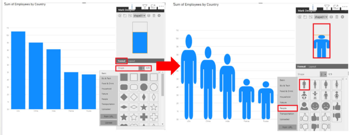
From the Mark Designer, go to ‘Format’ and select box adjacent to ‘Shape’. From the list of different shape types i.e., Basic, Biz & Tech, Food & Drink, Household, Nature, People, Transportation, Uploaded.  

Choose any one from the list. Here, we will choose ‘People’ from the of first icon. Once chosen, you will be able to see the updated icon as highlighted in the image below.

Step 4.2: Changing Chart Type to Bar and Enabling Multiple Units

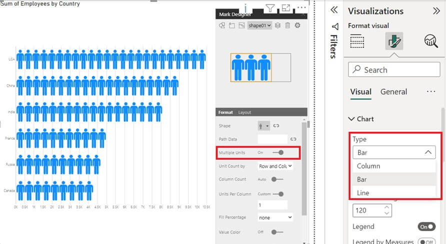
From the visualisations pane, we will need to format the viz as this is by default the ‘column’ type. For this, change the ‘Column’ type to ‘Bar’ type to have icons in the horizontal format whereas the column type will allow only one icon for each category in the vertically format.

Also, we will need to turn on the ‘Multiple Units’ ON as it will allow to have number of icons spread according to the range of measure value – from min to max.

The new look of the viz will be as below –

Step 4.3: Customizing Icon Colors

To change the color of the icon, turn ON the ‘Value Color’ option as shown in the image below. The default color will now change to green.

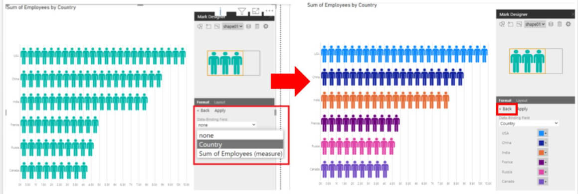
To change the same into multiple shades for each category, click on the small icon i.e., ‘Value Color Data-Binding’ which is adjacent to the color shade.

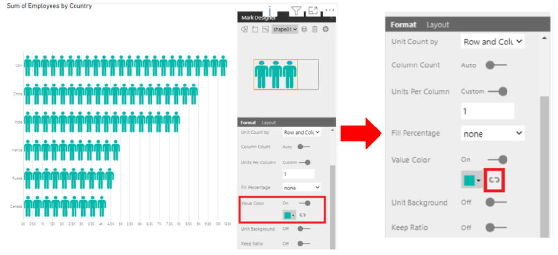
After this, you will see a bunch of options having ‘None’ selected by default, the Country (which is the category here) and the measure (which is sum of the value from employee field – this counts the number of employees here).

Select the category i.e., ‘Country’ and click ‘Apply’ to apply the changes made. As soon as the changes are applied, you will be able to see the changes

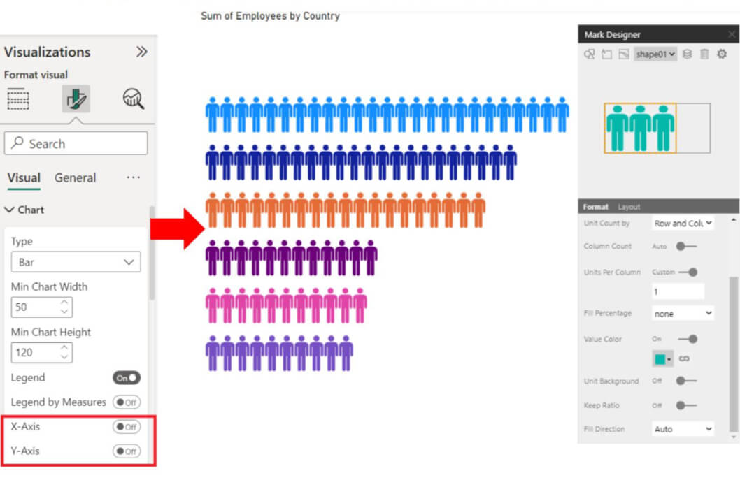
Step 5: Adjusting Axis and Data Labels

Now, that our infographic viz is almost ready, we will need to turn off the X and Y axis and place the data labels instead to the extreme right side.

Step 5.1: Disabling X-axis and Y-axis

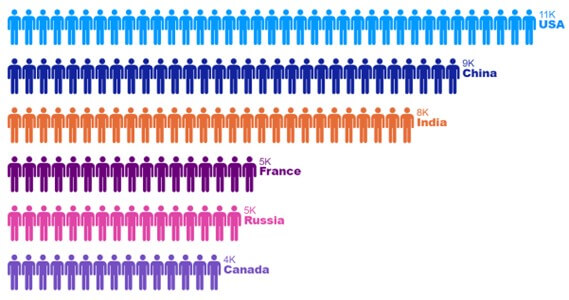
To accomplish that, go to the formatting option in the visualisations pane and under ‘Chart’. There you will see the option – X-axis and Y-axis. Turn OFF the buttons for both the axis. The viz will look like this –

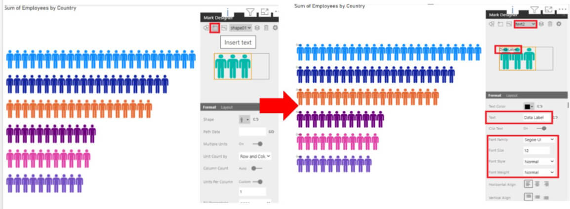
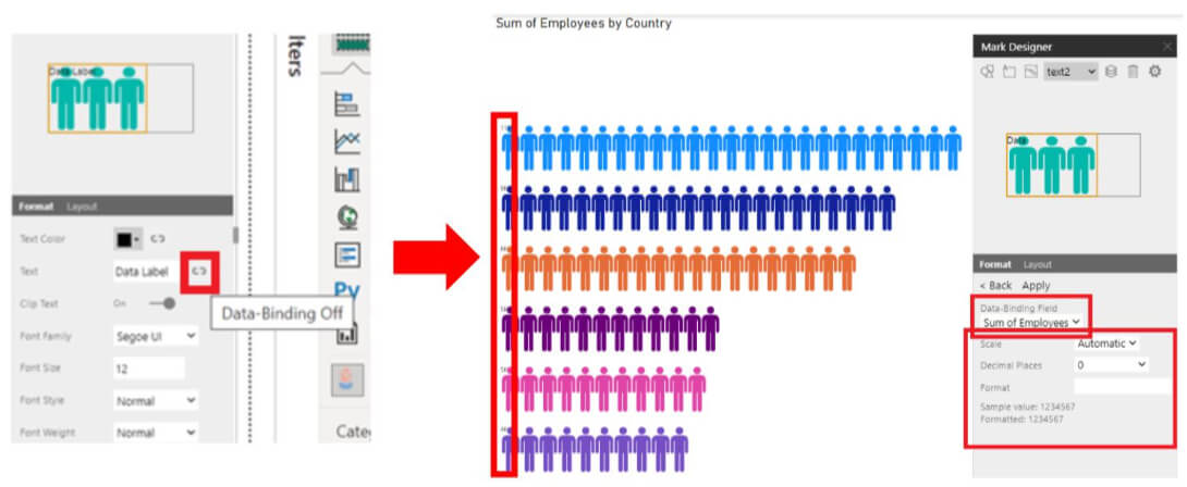
Step 5.2: Adding and Formatting Data Labels

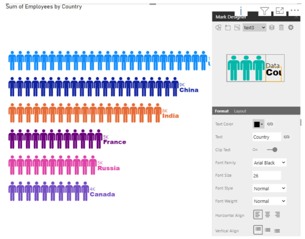
To insert the data labels, we will need to insert a text. By clicking on the second icon from the top, you will be able to add the text. The moment you click on the icon, it will show the name as ‘text2’ and you can even name the text to know what’s there in this text. Here, we will name this text as ‘Data Label’. The formatting of the text can also be done like font style, font size, alignment, color change, etc.

Step 6: Finalizing the Chart and Layout

For now, since we have not defined any text in the ‘text2’, hence, the name of the data label we added will be shown here. To add the text for ‘text02’, where in this case it will be the number of employees for each country, we will need to select the ‘Text Data Binding’ option which is present on the right side of ‘Data Label’.

After this, you will see Data-Binding field option. Select the measure (here employee count) and do the data label formatting as required. By doing this, the data labels in small size for each category will be visible.

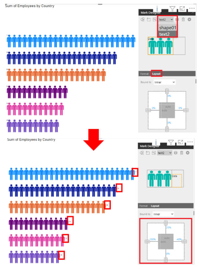
You will need to now align these labels to the extreme right position.

Step 6.1: Adjusting Data Label Alignment

Now, select the ‘Text2’ from top and go to ‘Layout’ option. Under this option, you will see the alignment settings for the text you selected. You can do the layout setting for the text (‘Text02’) according to the place you want to put the data label to. We will be placing it to extreme end. Hence, the layout setting will be done accordingly. By default, it will be 0% for all.

Note – You can switch to any already added shape/text to edit them for layout settings.

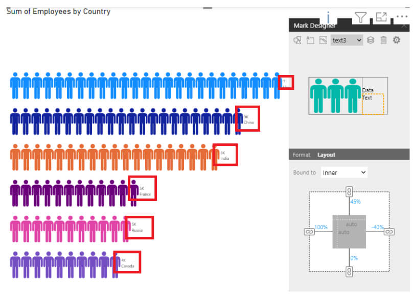
Step 6.2: Adding Category Labels

Now, add the category label in the similar manner. Add the text, a new text as ‘Text3’ will get added.

Add the ‘Text Data Binding’ field for this text – add the country category here. You will see the country label on the y-axis initially. Provide the layout to this text in the same way as done for the ‘Text2’ data label by following the steps from 12 to 14. Note that, you will need to add this data category label just below the previously added data label (count of employees). For this, you will need to make changes in the layout option accordingly.

Step 6.3: Formatting Text Colors and Styles

Now, that you have added both the data labels, the color of these data label needs to be changed. To accomplish this, you will need to select one text at a time. Select ‘Text2’ and go to ‘Text Color Data Binding’ option. Select ‘Country’ and finally apply the settings. The default colors for each country category will be replicated for the ‘Text2’ data label. Click on ‘Back’ button to go back to formatting and change the font size of 20 for ‘Text2’.

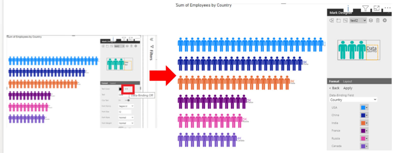
Perform the same step i.e., step-16 for the next text which is ‘Text3’. You should see –

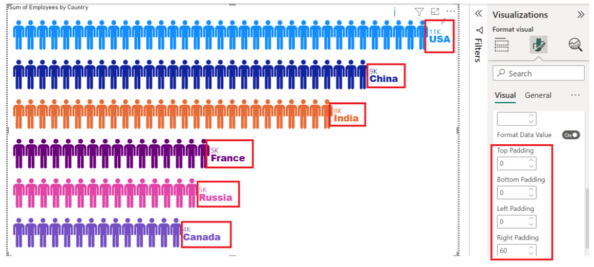
Step 7: Applying Padding and Title Formatting

Finally, use the padding options from the format section of the visualizations pane for this chart so that the data labels are in line.

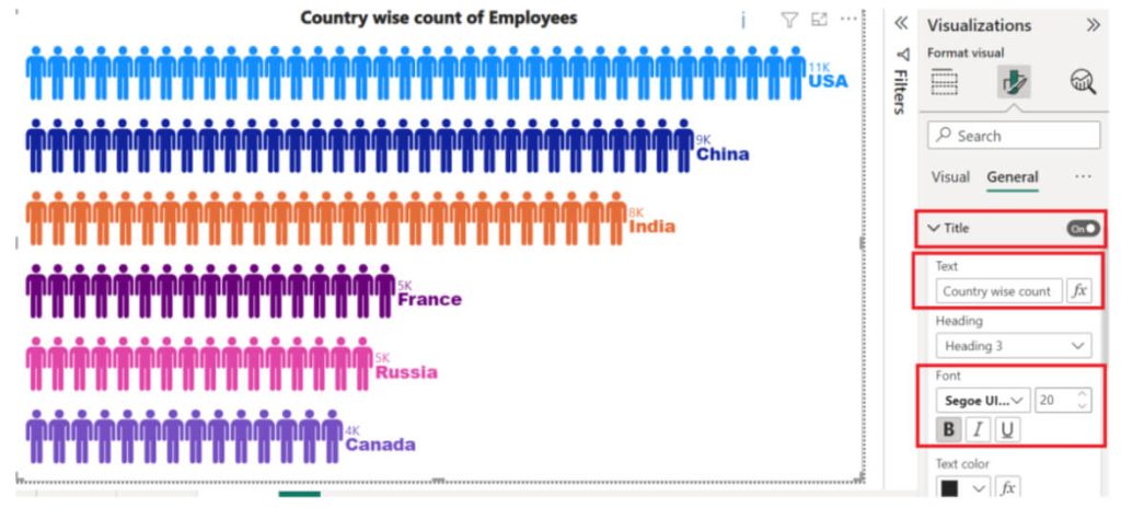
Step 7.1: Formatting the Chart Title 

Change the default title to ‘Country wise count of Employees’ from the format section and format the font size and font style as per the requirement of the title added.

Create Eye-Catching Visuals with Power BI’s Infographic Designer

The final output of infographic designer chart will look like below after cleaning up.